If you want to be a power user of MS Excel, you must master the most useful Excel formulas of Excel. To be frank, it is not an easy task for all as the functions are a lot in numbers.
One trick can help you!
102 Most Useful Excel Formulas with Examples
A. IS FUNCTIONS
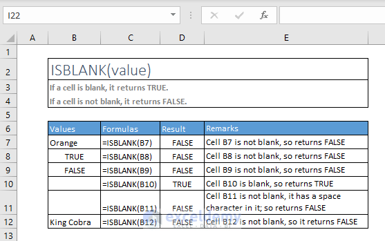
1. ISBLANK
=ISBLANK(value)
If a cell is blank, it returns TRUE. If a cell is not blank, it returns FALSE.
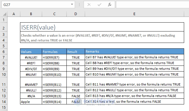
2. ISERR
=ISERR(value)
Checks whether a value is an error (#VALUE!, #REF!, #DIV/0!, #NUM!, #NAME?, or #NULL!) excluding #N/A, and returns TRUE or FALSE
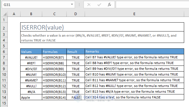
3. ISERROR
=ISERROR(value)
Checks whether a value is an error (#N/A, #VALUE!, #REF!, #DIV/0!, #NUM!, #NAME?, or #NULL!), and returns TRUE or FALSE
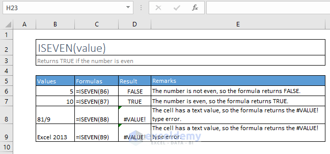
4. ISEVEN
=ISEVEN(value)
Returns TRUE if the number is even
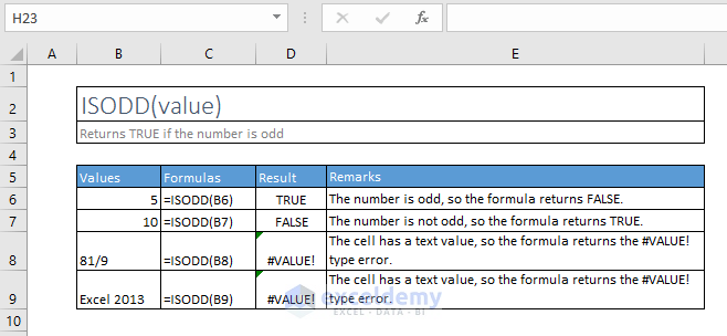
5. ISODD
=ISODD(value)
Returns TRUE if the number is odd
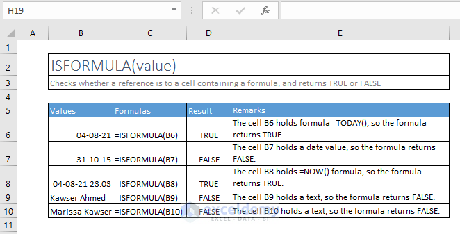
6. ISFORMULA
=ISFORMULA(value)
Checks whether a reference is to a cell containing a formula, and returns TRUE or FALSE
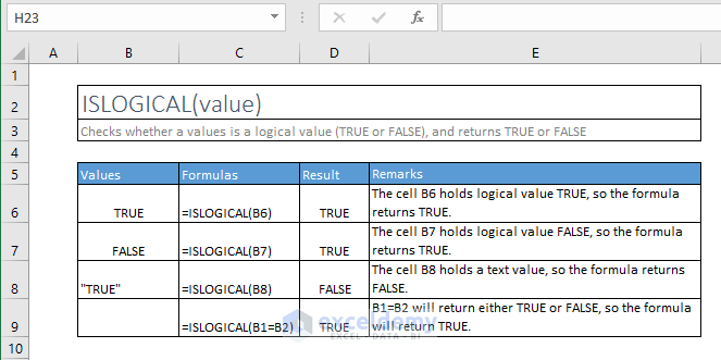
7. ISLOGICAL
=ISLOGICAL(value)
Checks whether a value is a logical value (TRUE or FALSE), and returns TRUE or FALSE
8. ISNA
=ISNA(value)
Checks whether a value is #N/A, and returns TRUE or FALSE

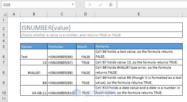
9. ISNUMBER
=ISNUMBER(value)
Checks whether a value is a number, and returns TRUE or FALSE
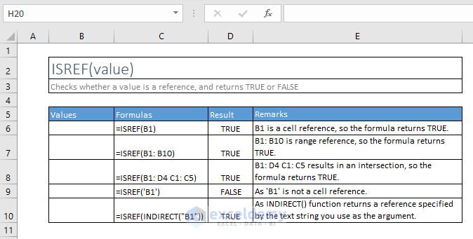
10. ISREF
=ISREF(value)
Checks whether a value is a reference, and returns TRUE or FALSE
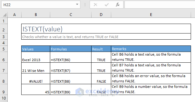
11. ISTEXT
=ISTEXT(value)
Checks whether a value is text, and returns TRUE or FALSE
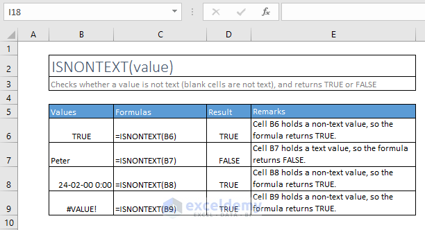
12. ISNONTEXT
=ISNONTEXT(value)
Checks whether a value is not text (blank cells are not text), and returns TRUE or FALSE
B. CONDITIONAL FUNCTIONS
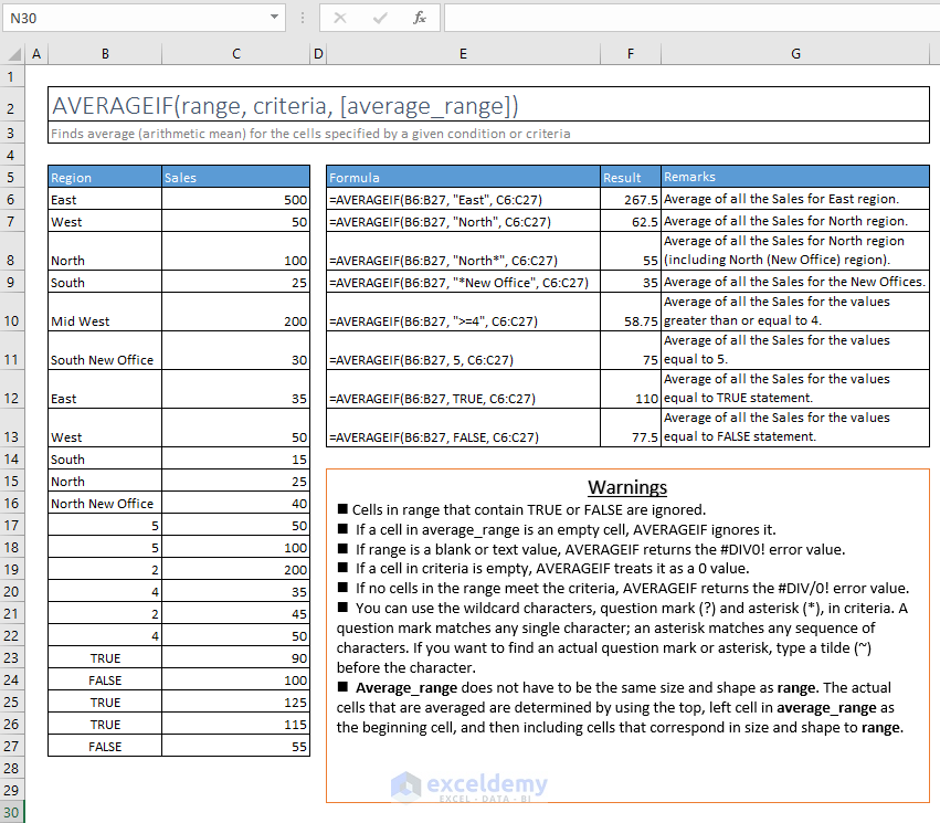
13. AVERAGEIF
=AVERAGEIF(range, criteria, [average_range])
Finds average (arithmetic mean) for the cells specified by a given condition or criteria
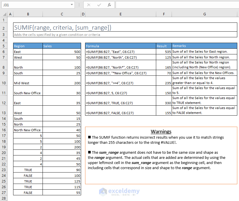
14. SUMIF
=SUMIF(range, criteria, [sum_range])
Adds the cells specified by a given condition or criteria
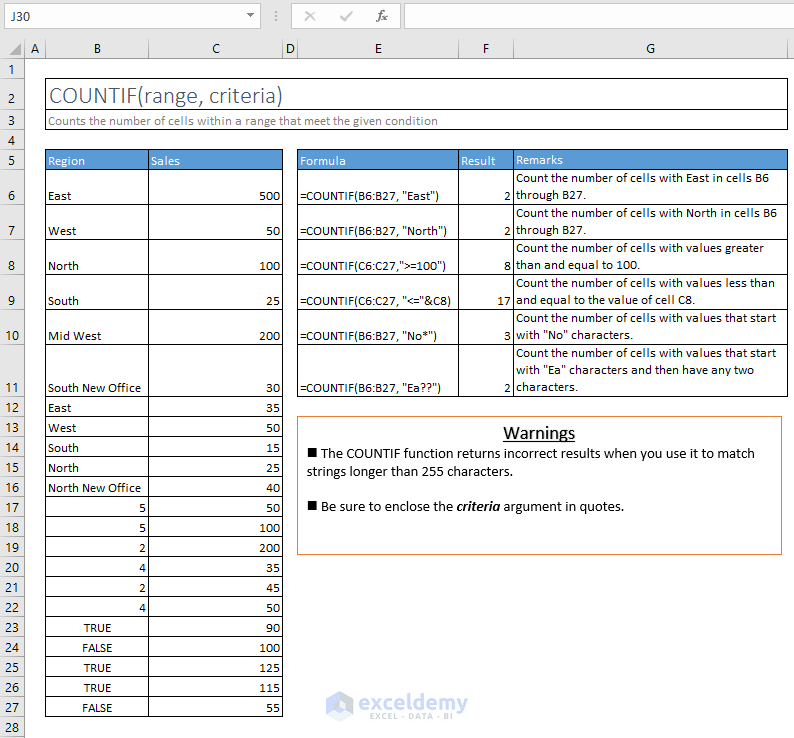
15. COUNTIF
=COUNTIF(range, criteria)
Counts the number of cells within a range that meet the given condition
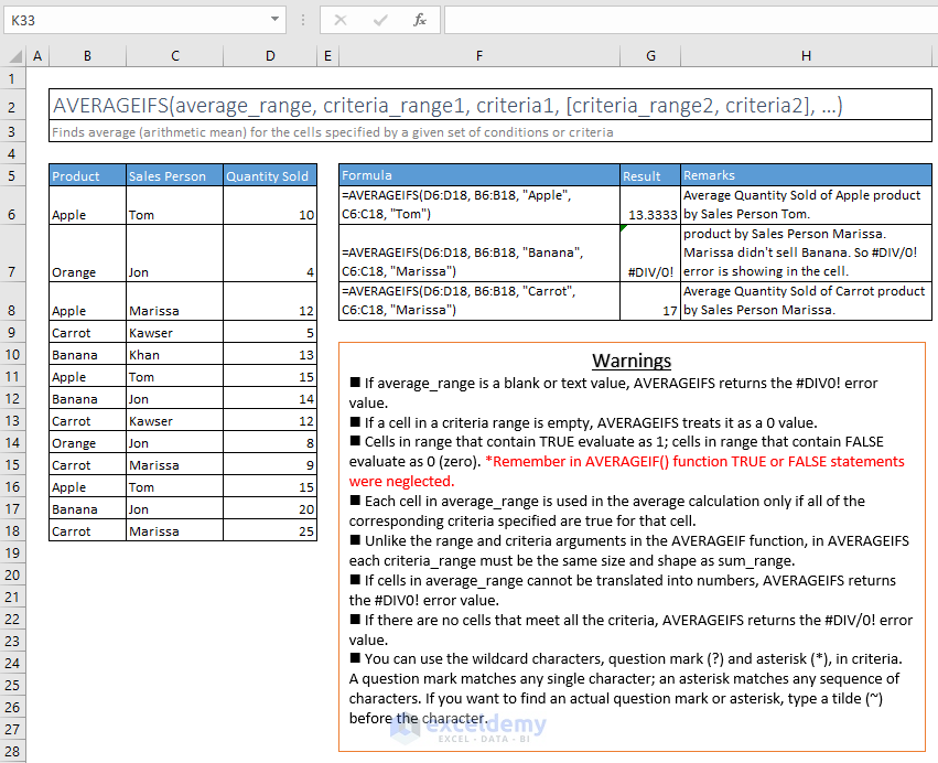
16. AVERAGEIFS
=AVERAGEIFS(average_range, criteria_range1, criteria1, [criteria_range2, criteria2], …)
Finds average (arithmetic mean) for the cells specified by a given set of conditions or criteria
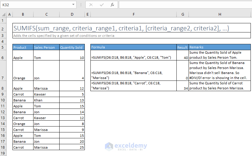
17. SUMIFS
=SUMIFS(sum_range, criteria_range1, criteria1, [criteria_range2, criteria2], …)
Adds the cells specified by a given set of conditions or criteria
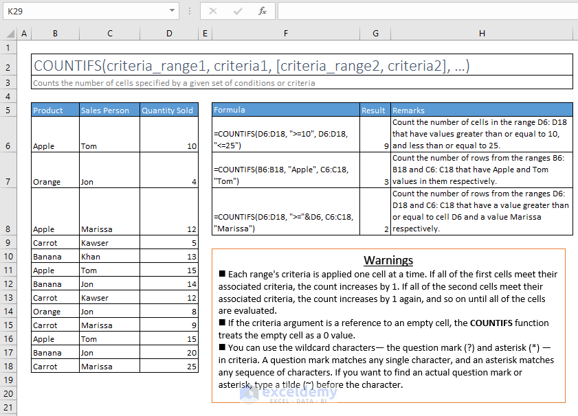
18. COUNTIFS
=COUNTIFS(criteria_range1, criteria1, [criteria_range2, criteria2], …)
Counts the number of cells specified by a given set of conditions or criteria
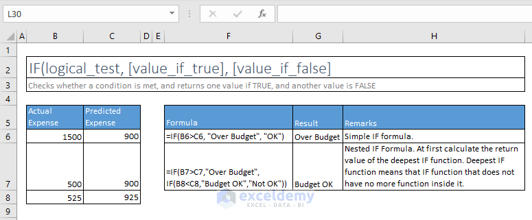
19. IF
=IF(logical_test, [value_if_true], [value_if_false]
Checks whether a condition is met, and returns one value if TRUE, and another value is FALSE
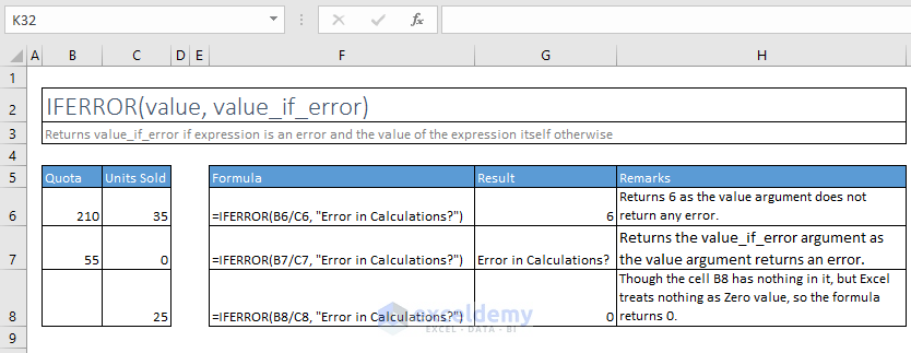
20. IFERROR
=IFERROR(value, value_if_error)
Returns value_if_error if the expression is an error and the value of the expression itself otherwise
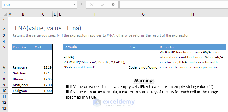
21. IFNA
=IFNA(value, value_if_na)
Returns the value you specify if the expression resolves to #N/A, otherwise returns the result of the expression
C. MATHEMATICAL FUNCTIONS
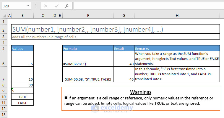
22. SUM
=SUM(number1, [number2], [number3], [number4], …)
Adds all the numbers in a range of cells
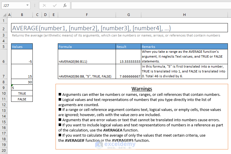
23. AVERAGE
=AVERAGE(number1, [number2], [number3], [number4], …)
Returns the average (arithmetic means) of its arguments, which can be numbers or names, arrays, or references that contain numbers
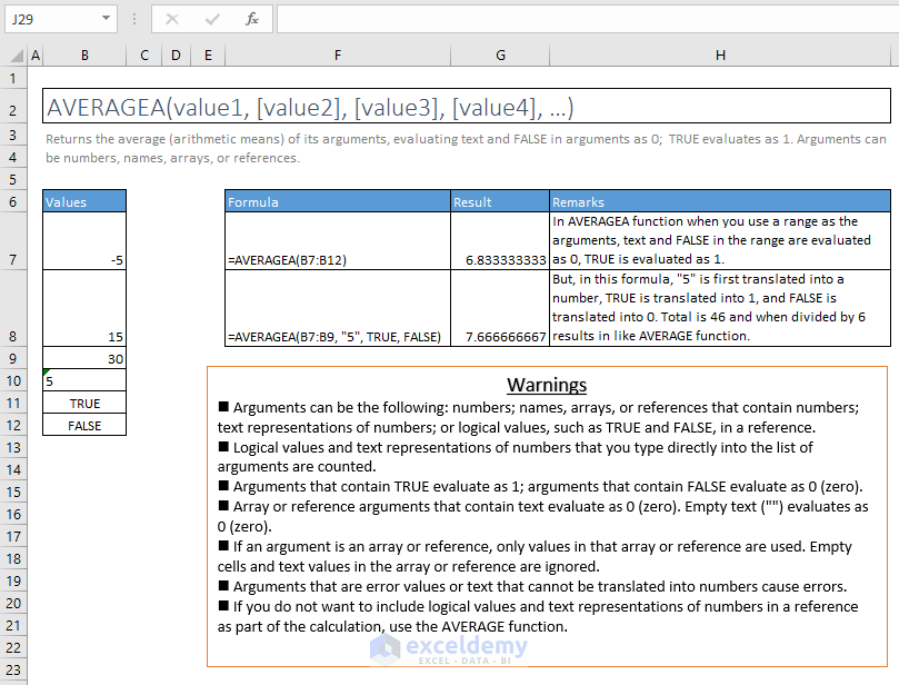
24. AVERAGEA
=AVERAGEA(value1, [value2], [value3], [value4], …)
Returns the average (arithmetic means) of its arguments, evaluating text and FALSE in arguments as 0; TRUE evaluates as 1. Arguments can be numbers, names, arrays, or references.
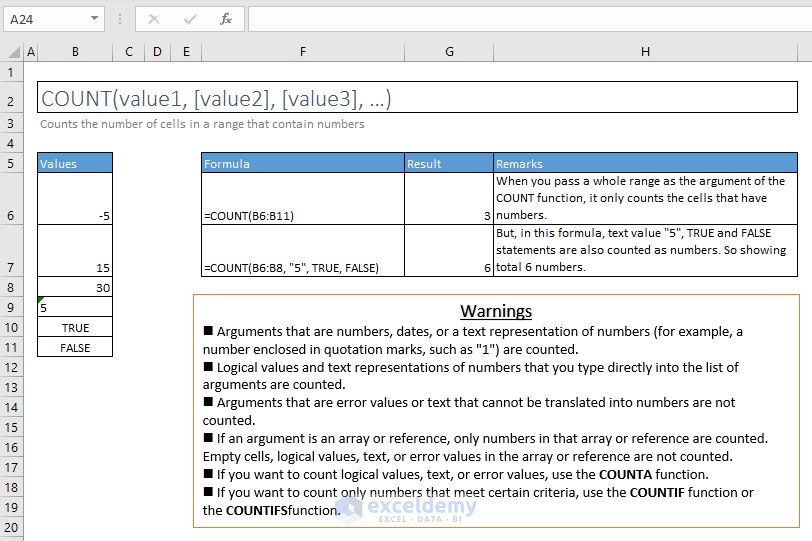
25. COUNT
=COUNT(value1, [value2], [value3], …)
Count the number of cells in a range that contain numbers
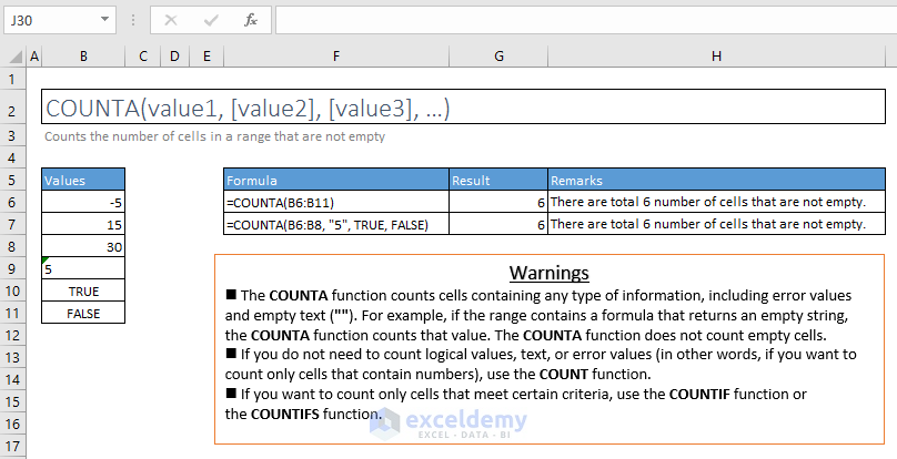
26. COUNTA
=COUNTA(value1, [value2], [value3], …)
Counts the number of cells in a range that are not empty
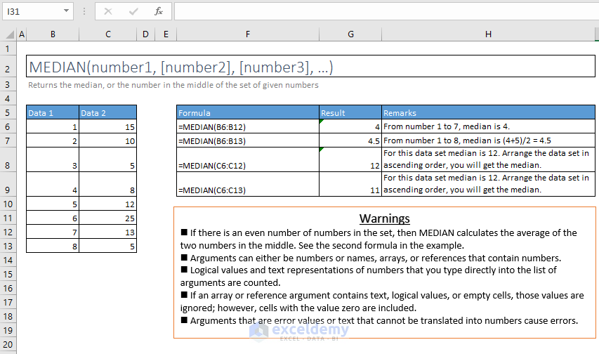
27. MEDIAN
=MEDIAN(number1, [number2], [number3], …)
Returns the median, or the number in the middle of the set of given numbers
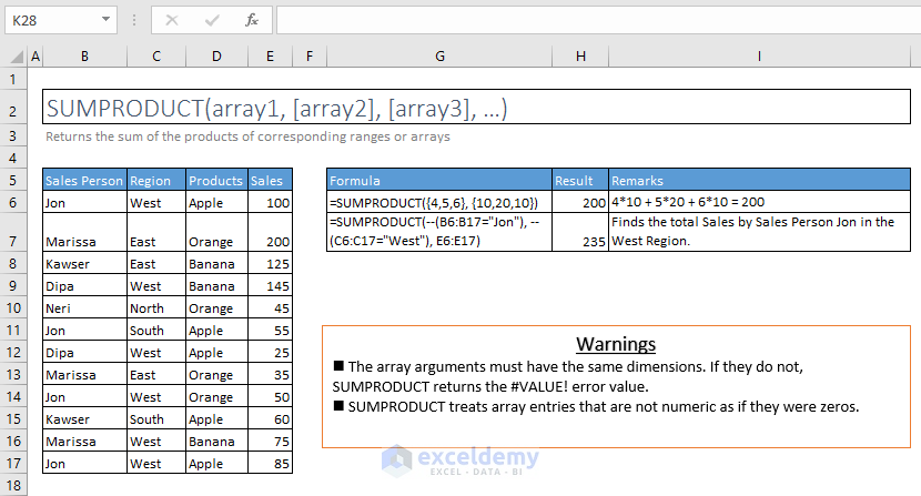
28. SUMPRODUCT
=SUMPRODUCT(array1, [array2], [array3], …)
Returns the sum of the products of corresponding ranges or arrays
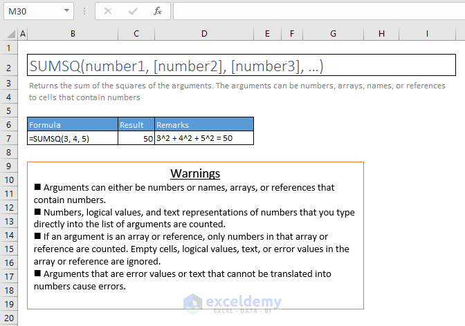
29. SUMSQ
=SUMSQ(number1, [number2], [number3], …)
Returns the sum of the squares of the arguments. The arguments can be numbers, arrays, names, or references to cells that contain numbers
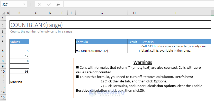
30. COUNTBLANK
=COUNTBLANK(range)
Counts the number of empty cells in a range
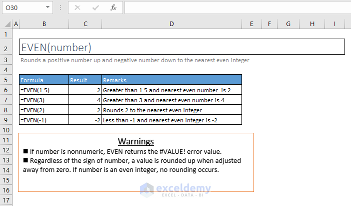
31. EVEN
=EVEN(number)
Rounds a positive number up and negative number down to the nearest even integer
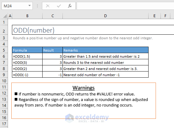
32. ODD
=ODD(number)
Rounds a positive number up and negative number down to the nearest odd integer.
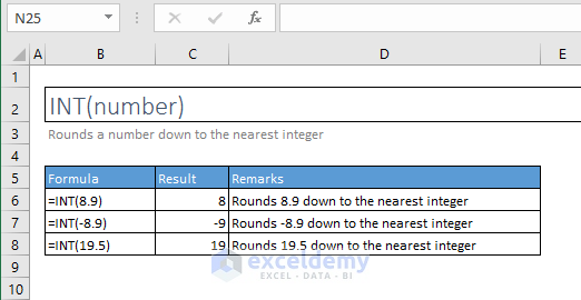
33. INT
=INT(number)
Rounds a number down to the nearest integer
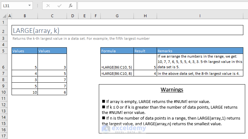
34. LARGE
=LARGE(array, k)
Returns the k-th largest value in a data set. For example, the fifth-largest number
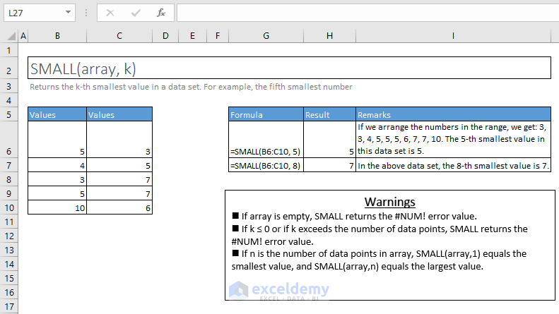
35. SMALL
=SMALL(array, k)
Returns the k-th smallest value in a data set. For example, the fifth smallest number
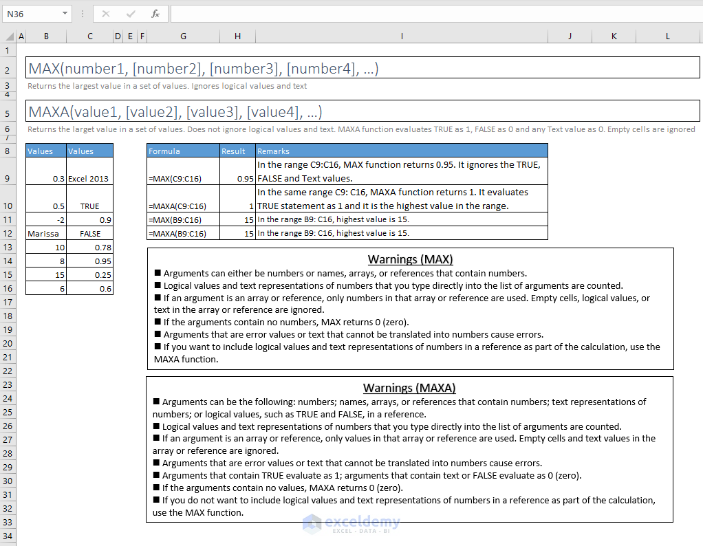
36. MAX & MAXA
=MAX(number1, [number2], [number3], [number4], …)
Returns the largest value in a set of values. Ignores logical values and text
=MAXA(value1, [value2], [value3], [value4], …)
Returns the largest value in a set of values. Do not ignore logical values and text. MAXA function evaluates TRUE as 1, FALSE as 0, and any Text value as 0. Empty cells are ignored
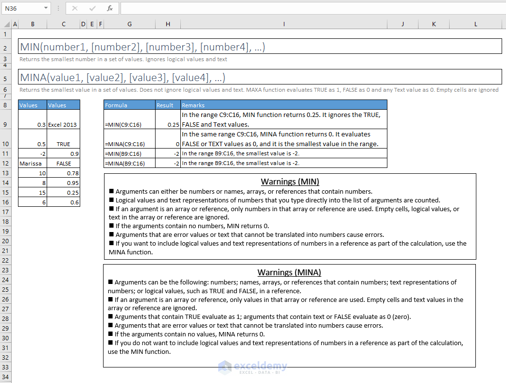
37. MIN & MINA
=MIN(number1, [number2], [number3], [number4], …)
Returns the smallest number in a set of values. Ignores logical values and text
=MINA(value1, [value2], [value3], [value4], …)
Returns the smallest value in a set of values. Do not ignore logical values and text. MAXA function evaluates TRUE as 1, FALSE as 0, and any Text value as 0. Empty cells are ignored
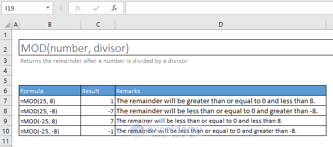
38. MOD
=MOD(number, divisor)
Returns the remainder after a number is divided by a divisor
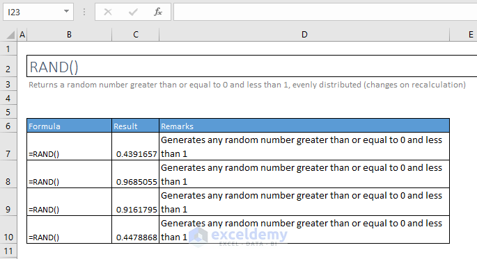
39. RAND
=RAND()
Returns a random number greater than or equal to 0 and less than 1, evenly distributed (changes on recalculation)
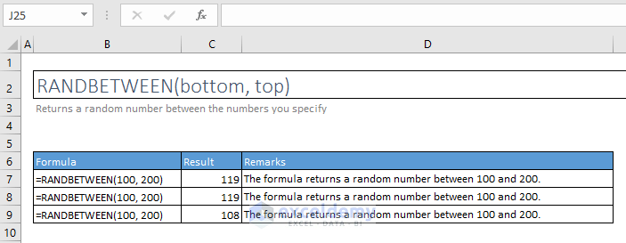
40. RANDBETWEEN
=RANDBETWEEN(bottom, top)
Returns a random number between the numbers you specify
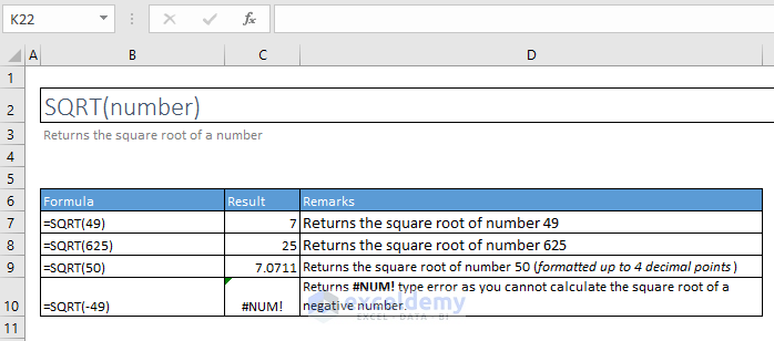
41. SQRT
=SQRT(number)
Returns the square root of a number
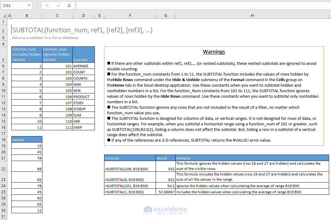
42. SUBTOTAL
=SUBTOTAL(function_num, ref1, [ref2], [ref3], …)
Returns a subtotal in a list or database
D. FIND & SEARCH FUNCTIONS
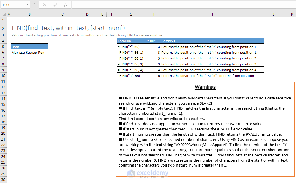
43. FIND
=FIND(find_text, within_text, [start_num])
Returns the starting position of one text string within another text string. FIND is case-sensitive
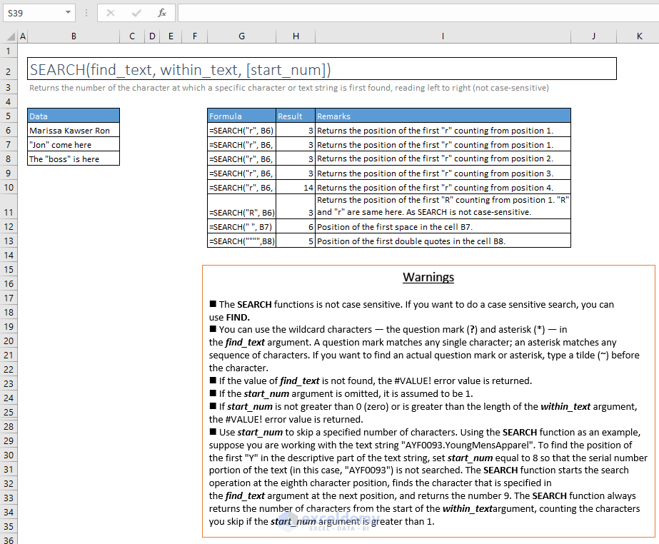
44. SEARCH
=SEARCH(find_text, within_text, [start_num])
Returns the number of the character at which a specific character or text string is first found, reading left to right (not case-sensitive)
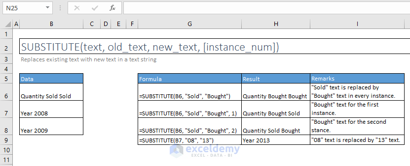
45. SUBSTITUTE
=SUBSTITUTE(text, old_text, new_text, [instance_num])
Replaces existing text with new text in a text string
46. REPLACE
=REPLACE(old_text, start_num, num_chars, new_text)
Replaces part of a text string with a different text string

E. LOOKUP FUNCTIONS
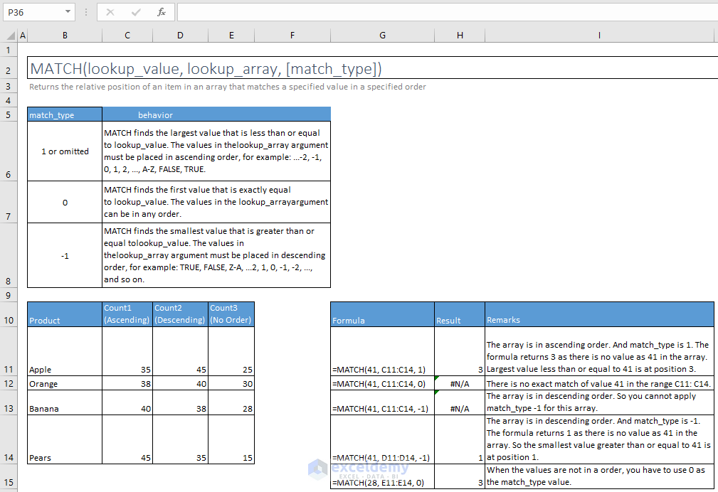
47. MATCH
=MATCH(lookup_value, lookup_array, [match_type])
Returns the relative position of an item in an array that matches a specified value in a specified order
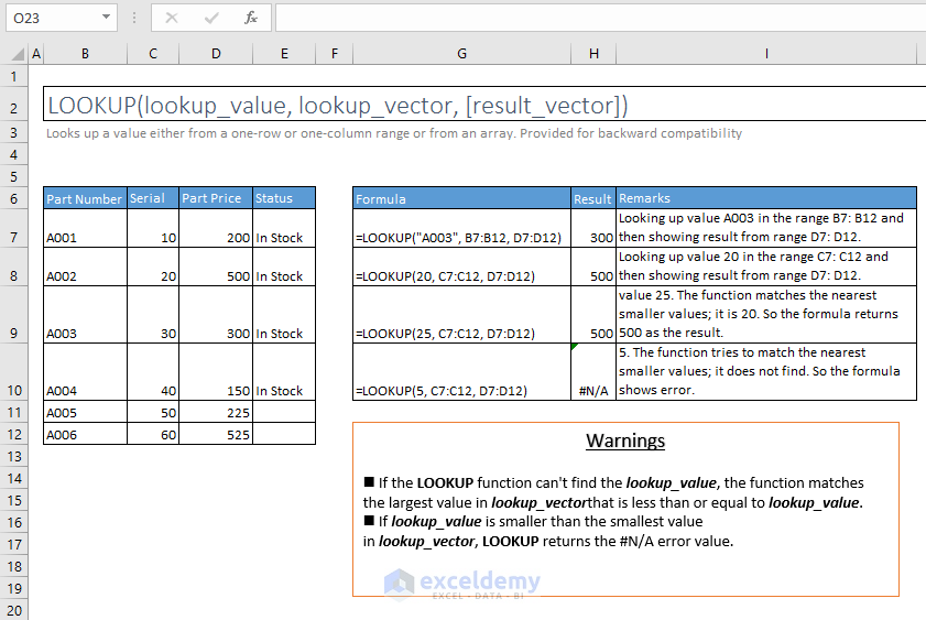
48. LOOKUP
=LOOKUP(lookup_value, lookup_vector, [result_vector])
Looks up a value either from a one-row or one-column range or from an array. Provided for backward compatibility
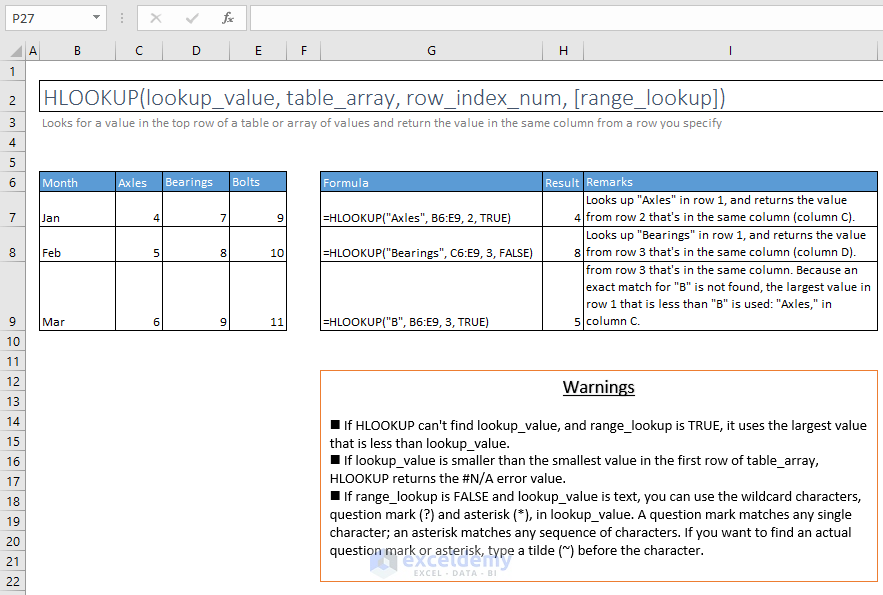
49. HLOOKUP
=HLOOKUP(lookup_value, table_array, row_index_num, [range_lookup])
Looks for a value in the top row of a table or array of values and return the value in the same column from a row you specify
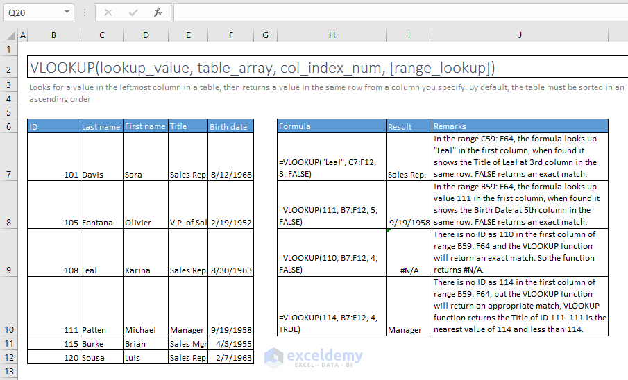
50. VLOOKUP
=VLOOKUP(lookup_value, table_array, col_index_num, [range_lookup])
Looks for a value in the leftmost column in a table, then return a value in the same row from a column you specify. By default, the table must be sorted in an ascending order
F. REFERENCE FUNCTIONS
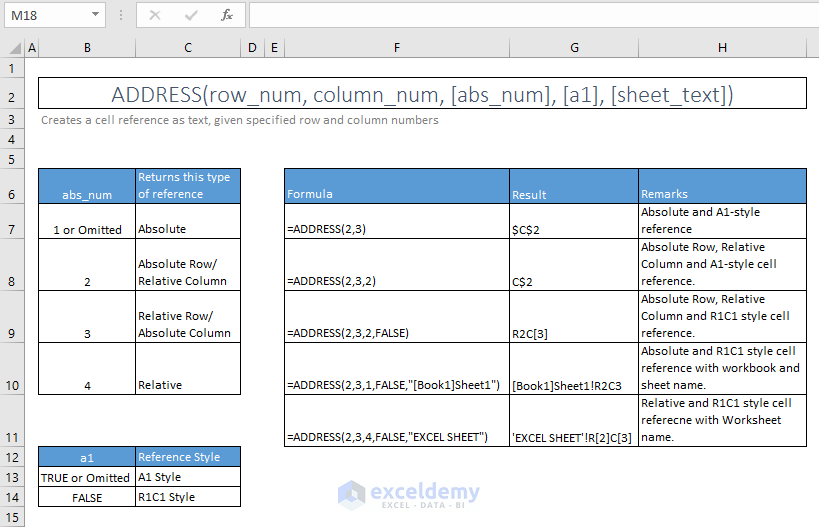
51. ADDRESS
=ADDRESS(row_num, column_num, [abs_num], [a1], [sheet_text])
Creates a cell reference as text, given specified row and column numbers
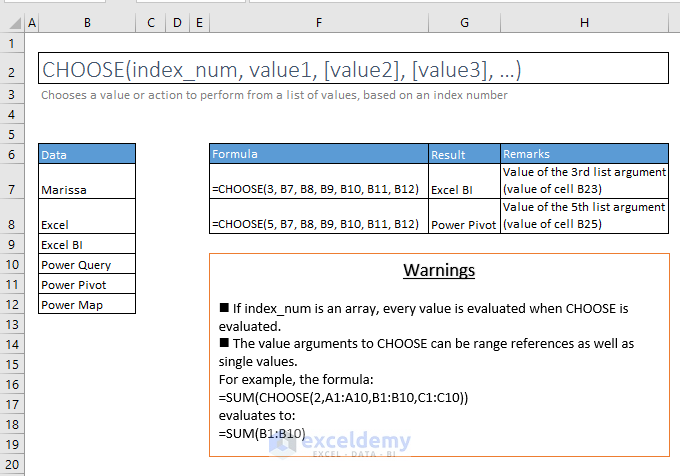
52. CHOOSE
=CHOOSE(index_num, value1, [value2], [value3], …)
Chooses a value or action to perform from a list of values, based on an index number
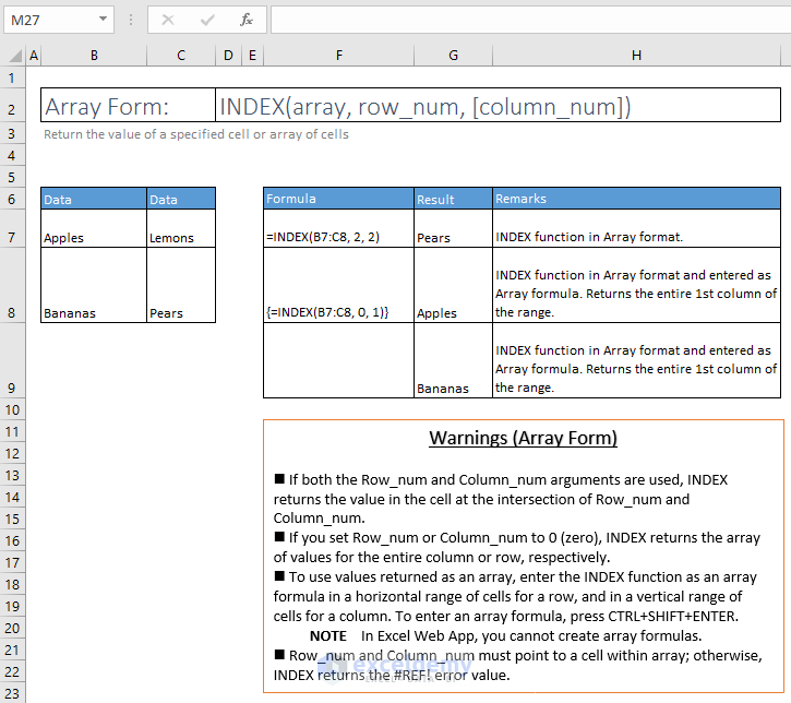
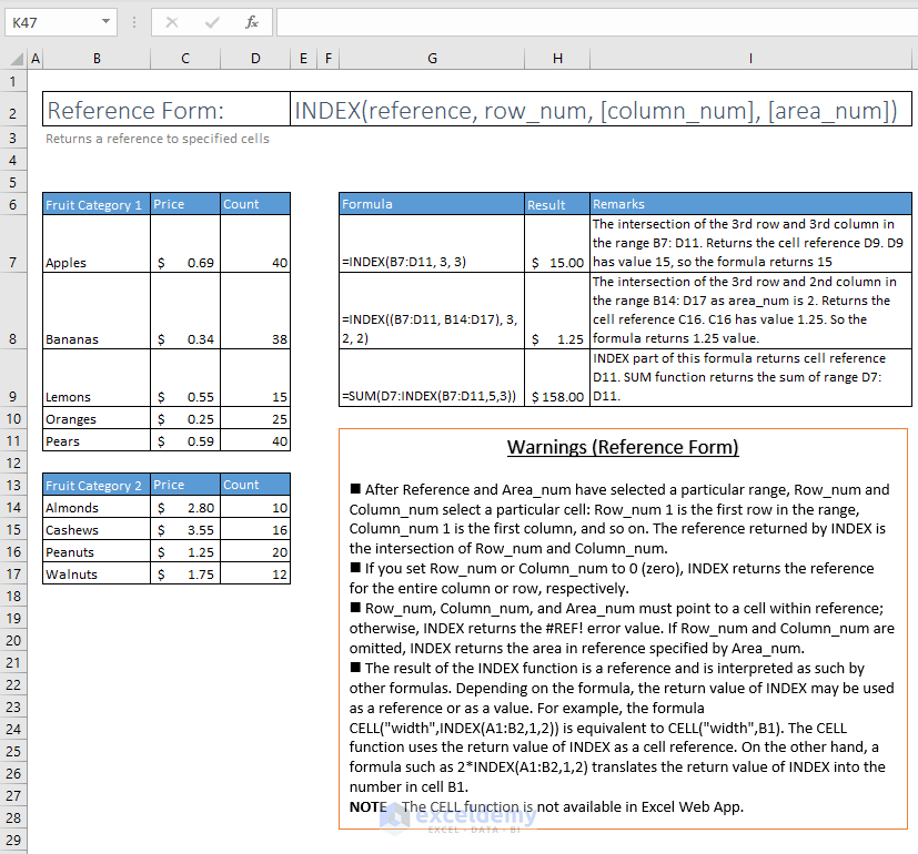
53. INDEX
Array Form: =INDEX(array, row_num, [column_num])
Return the value of a specified cell or array of cells
Reference Form: =INDEX(reference, row_num, [column_num], [area_num])
Returns a reference to specified cells
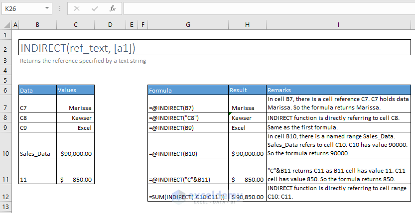
54. INDIRECT
=INDIRECT(ref_text, [a1])
Returns the reference specified by a text string
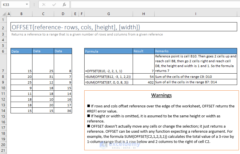
55. OFFSET
=OFFSET(reference- rows, cols, [height], [width])
Returns a reference to a range that is a given number of rows and columns from a given reference
G. DATE & TIME FUNCTIONS
56. DATE
=DATE(year, month, day)
Returns the number that represents the date in Microsoft Excel date-time code

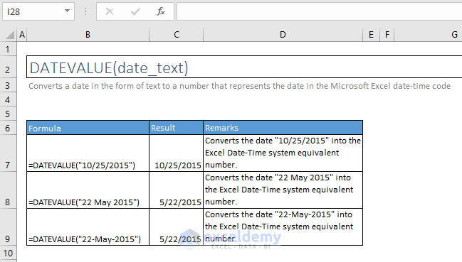
57. DATEVALUE
=DATEVALUE(date_text)
Converts a date in the form of text to a number that represents the date in the Microsoft Excel date-time code
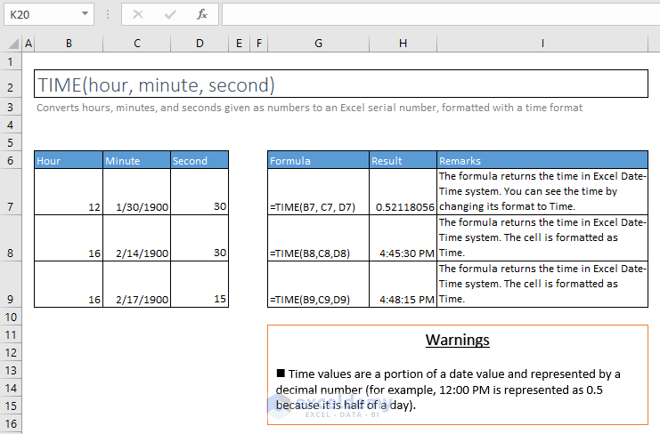
58. TIME
=TIME(hour, minute, second)
Converts hours, minutes, and seconds given as numbers to an Excel serial number, formatted with a time format
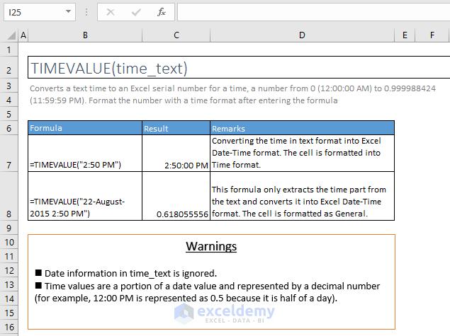
59. TIMEVALUE
=TIMEVALUE(time_text)
Converts a text time to an Excel serial number for a time, a number from 0 (12:00:00 AM) to 0.999988424 (11:59:59 PM). Format the number with a time format after entering the formula
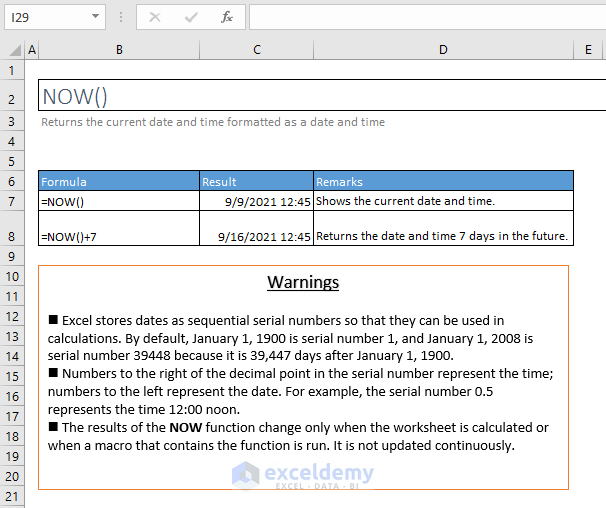
60. NOW
=NOW()
Returns the current date and time formatted as a date and time
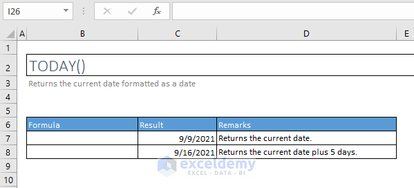
61. TODAY
=TODAY()
Returns the current date formatted as a date
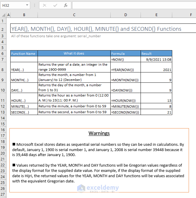
62. YEAR(), MONTH(), DAY(), HOUR(), MINUTE(), SECOND()
YEAR(), MONTH(), DAY(), HOUR(), MINUTE() and SECOND() Functions
All these functions take one argument: serial_number
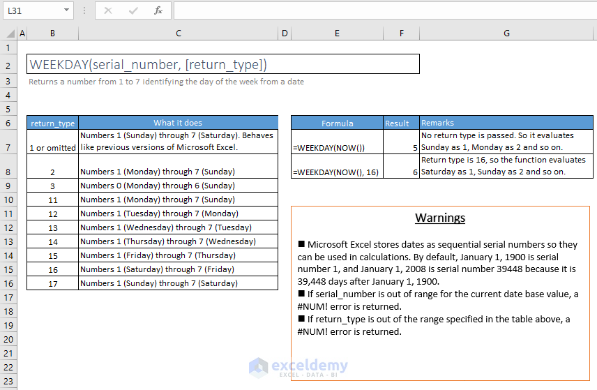
63. WEEKDAY
=WEEKDAY(serial_number, [return_type])
Returns a number from 1 to 7 identifying the day of the week from a date
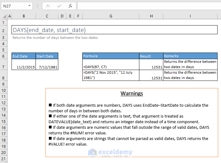
64. DAYS
=DAYS(end_date, start_date)
Returns the number of days between the two dates
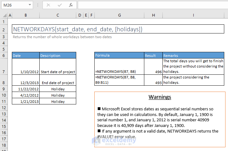
65. NETWORKDAYS
=NETWORKDAYS(start_date, end_date, [holidays])
Returns the number of whole workdays between two dates
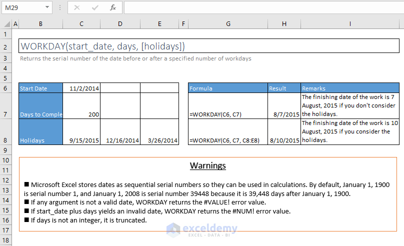
66. WORKDAY
=WORKDAY(start_date, days, [holidays])
Returns the serial number of the date before or after a specified number of workdays
H. MISCELLANEOUS FUNCTIONS
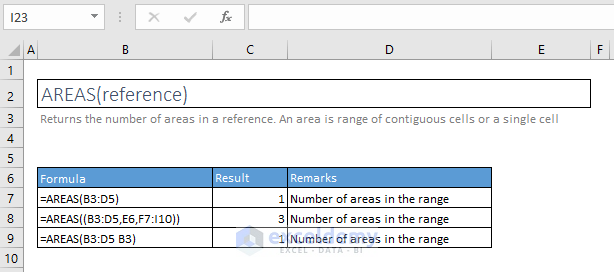
67. AREAS
=AREAS(reference)
Returns the number of areas in a reference. An area is a range of contiguous cells or a single cell
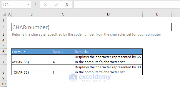
68. CHAR
=CHAR(number)
Returns the character specified by the code number from the character set for your computer
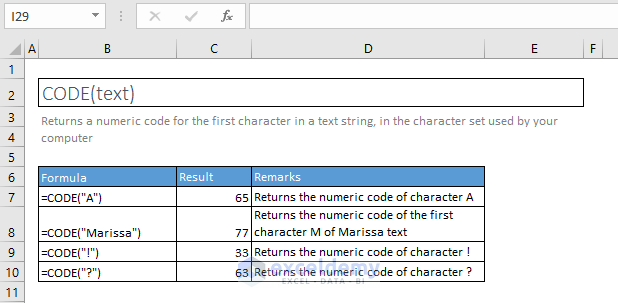
69. CODE
=CODE(text)
Returns a numeric code for the first character in a text string, in the character set used by your computer
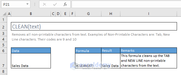
70. CLEAN
=CLEAN(text)
Removes all non-printable characters from text. Examples of Non-Printable Characters are Tab, New Line characters. Their codes are 9 and 10.
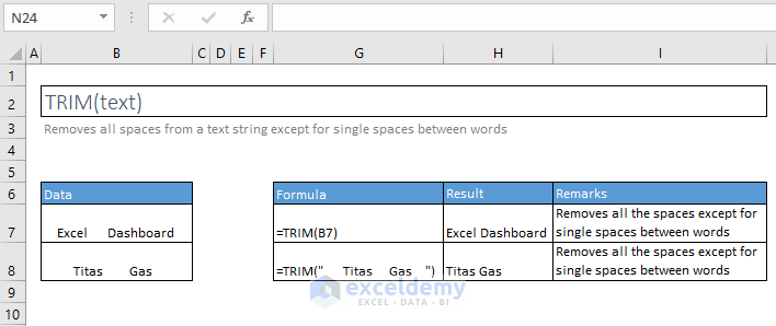
71. TRIM
=TRIM(text)
Removes all spaces from a text string except for single spaces between words
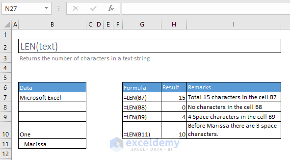
72. LEN
=LEN(text)
Returns the number of characters in a text string
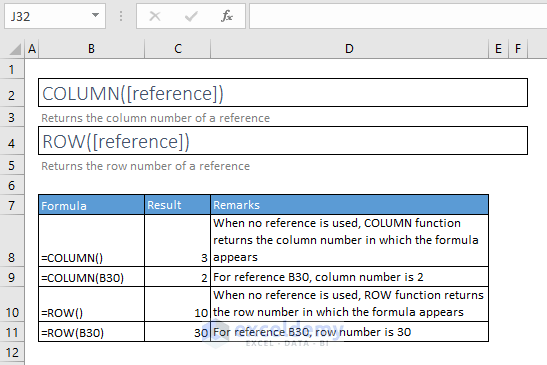
73. COLUMN() & ROW() Functions
=COLUMN([reference])
Returns the column number of a reference
=ROW([reference])
Returns the row number of a reference
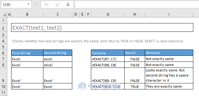
74. EXACT
=EXACT(text1, text2)
Checks whether two text strings are exactly the same, and returns TRUE or FALSE. EXACT is case-sensitive
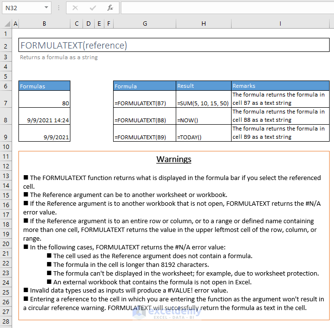
75. FORMULATEXT
=FORMULATEXT(reference)
Returns a formula as a string
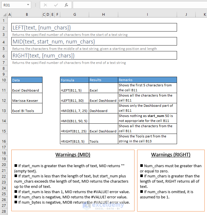
76. LEFT(), RIGHT(), and MID() Functions
=LEFT(text, [num_chars])
Returns the specified number of characters from the start of a text string
=MID(text, start_num, num_chars)
Returns the characters from the middle of a text string, given a starting position and length
=RIGHT(text, [num_chars])
Returns the specified number of characters from the end of a text string
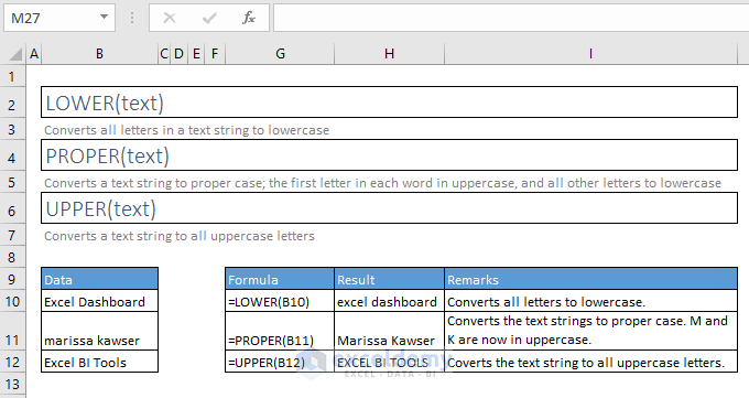
77. LOWER(), PROPER(), and UPPER() Functions
=LOWER(text)
Converts all letters in a text string to lowercase
=PROPER(text)
Converts a text string to proper case; the first letter in each word in uppercase, and all other letters to lowercase
=UPPER(text)
Converts a text string to all uppercase letters
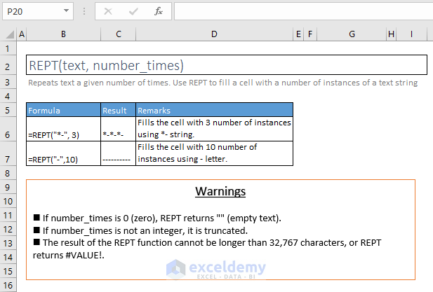
78. REPT
=REPT(text, number_times)
Repeats text a given number of times. Use REPT to fill a cell with a number of instances of a text string
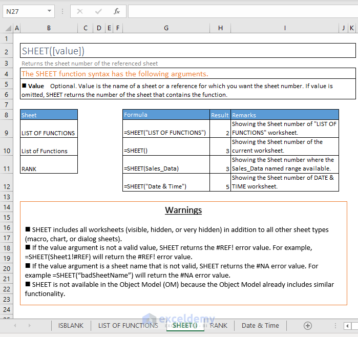
79. SHEET
=SHEET([value])
Returns the sheet number of the referenced sheet
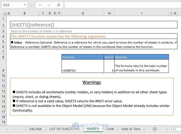
80. SHEETS
=SHEETS([reference])
Returns the number of sheets in a reference
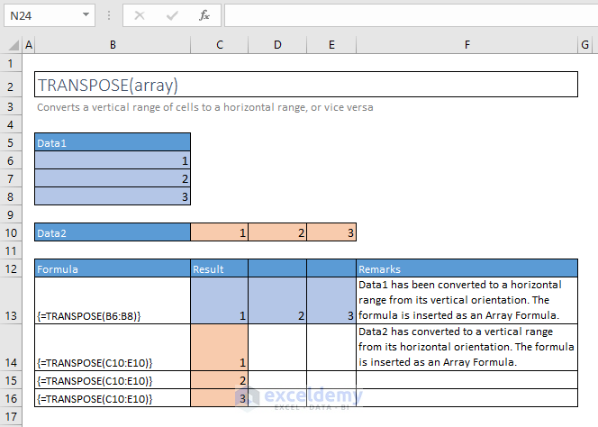
81. TRANSPOSE
=TRANSPOSE(array)
Converts a vertical range of cells to a horizontal range, or vice versa
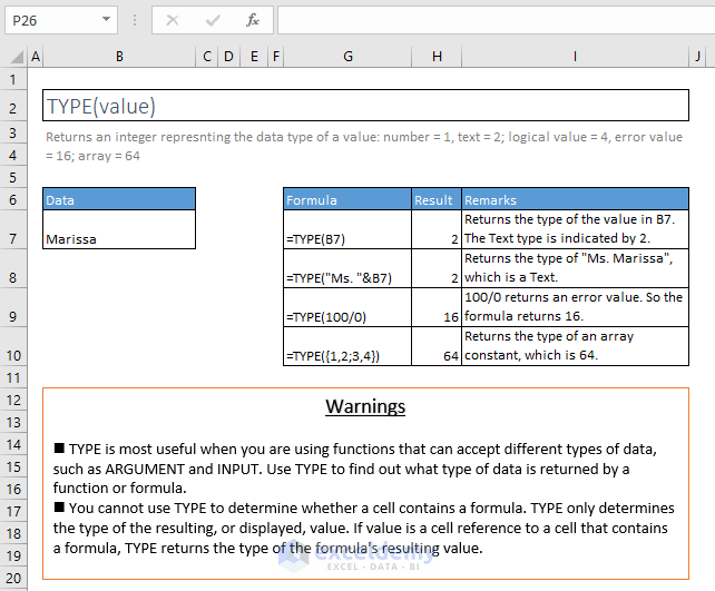
82. TYPE
=TYPE(value)
Returns an integer represnting the data type of a value: number = 1, text = 2; logical value = 4, error value = 16; array = 64
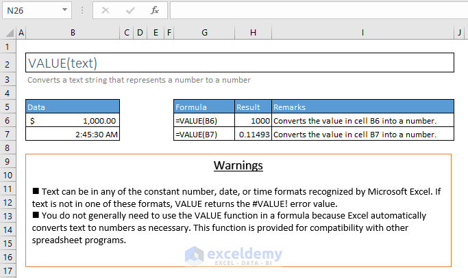
83. VALUE
=VALUE(text)
Converts a text string that represents a number to a number
I. RANK FUNCTIONS
84. RANK
=RANK(number, ref, [order])
This function is available for compatibility with Excel 2007 and others.
Returns the rank of a number in a list of numbers: its size relative to other values in the list
![]()
85. RANK.AVG
=RANK.AVG(number, ref, [order])
Returns the rank of a number in a list of numbers: its size relative to other values in the list; if more than one value has the same rank, the average rank is returned
![]()
86. RANK.EQ
=RANK.EQ(number, ref, [order])
Returns the rank of a number in a list of numbers: its size relative to other values in the list; if more than one value has the same rank, the top rank of that set of values is returned
![]()
J. LOGICAL FUNCTIONS
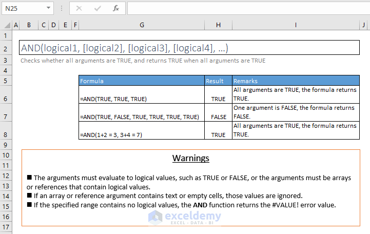
87. AND
=AND(logical1, [logical2], [logical3], [logical4], …)
Checks whether all arguments are TRUE, and returns TRUE when all arguments are TRUE
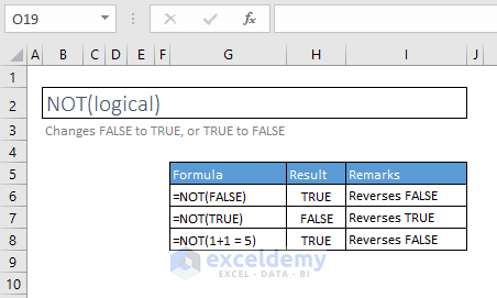
88. NOT
=NOT(logical)
Changes FALSE to TRUE, or TRUE to FALSE
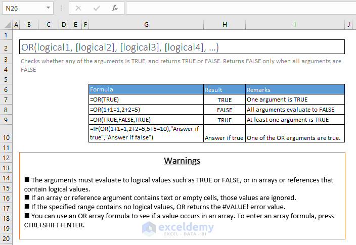
89. OR
=OR(logical1, [logical2], [logical3], [logical4], …)
Checks whether any of the arguments is TRUE, and returns TRUE or FALSE. Returns FALSE only when all arguments are FALSE
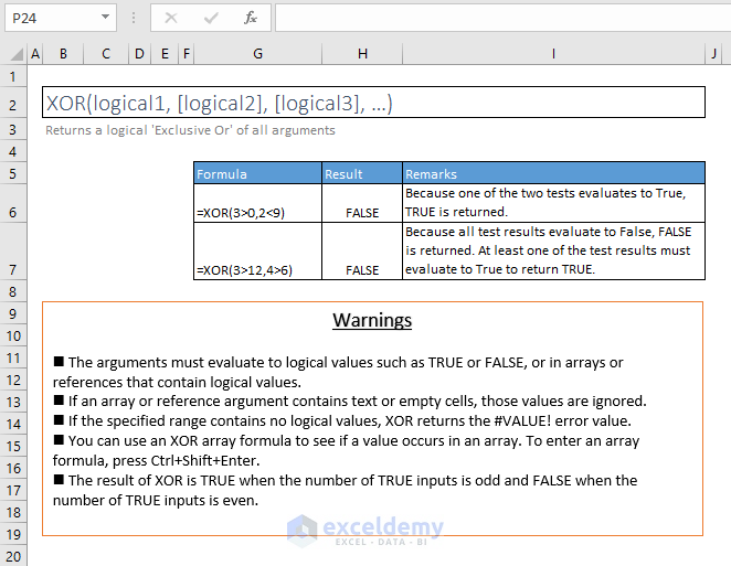
90. XOR
=XOR(logical1, [logical2], [logical3], …)
Returns a logical ‘Exclusive Or’ of all arguments